Day 91: Principal Component Analysis (PCA) Theory
Ready to move beyond basic prompts and start building production-ready AI? The AI Agent Mastery Course is a deep-dive, hands-on guide to architecting the next generation of intelligent systems. From mastering ReAct planning and self-healing logic to building complex multi-agent orchestrations, this curriculum bridges the gap between AI theory and real-world engineering. Don't just watch the AI revolution—build it. Join the community and start building today at aiamastery.substack.com.
What We’ll Build Today
A mathematical foundation for understanding PCA’s variance maximization principle
Implementation of covariance matrix computation and eigenvalue decomposition
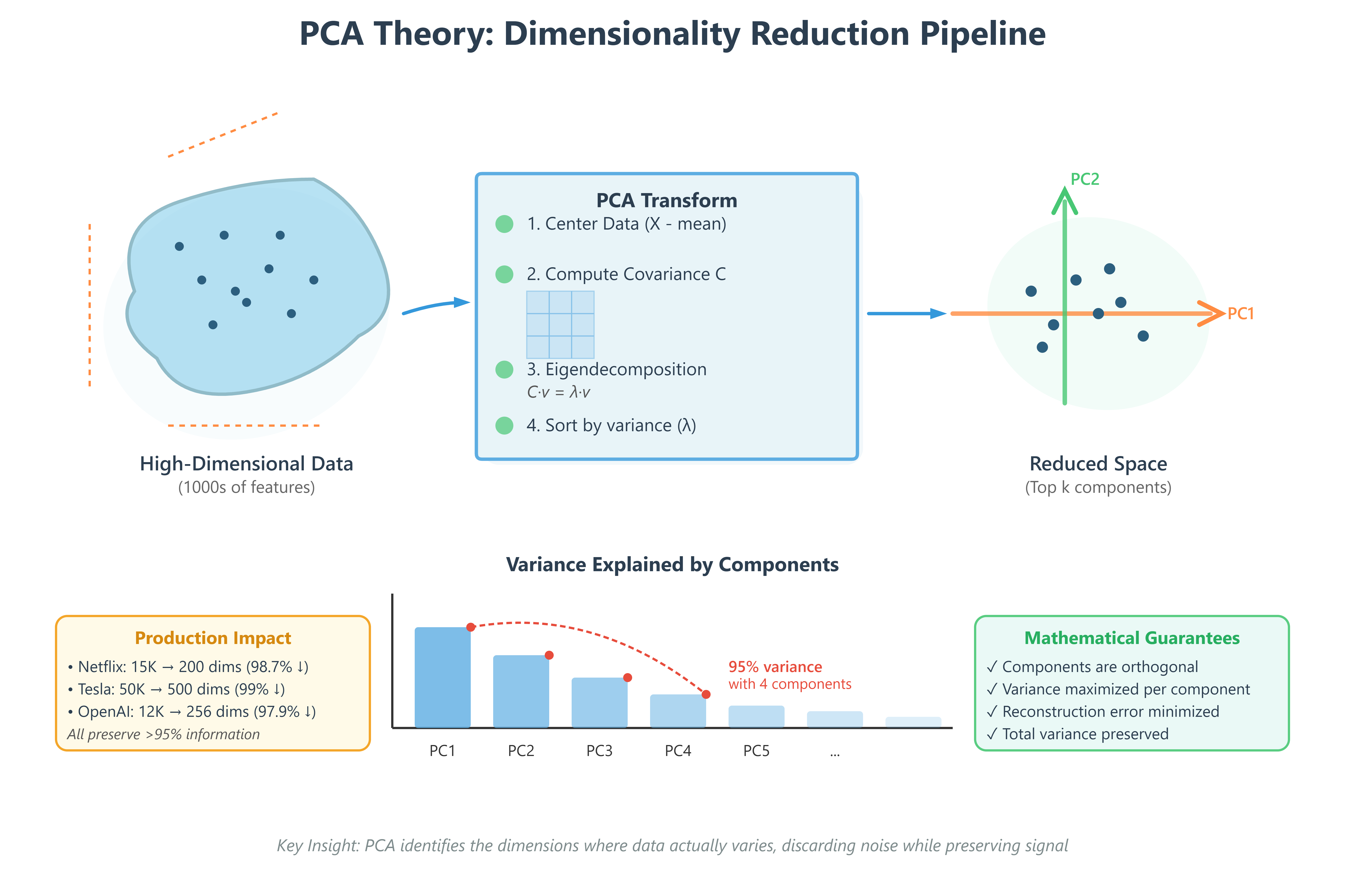
A visualization system showing how PCA transforms high-dimensional data
Production-grade testing suite validating mathematical correctness
Why This Matters: The Compression Engine Behind Modern AI
Every second, Netflix processes viewing data with 15,000+ features per user (watch history, pause points, rewind patterns, device types, time of day, etc.). Google Search analyzes documents with 100,000+ dimensional embeddings. Tesla’s vision system captures sensor data with 50,000+ features per frame. These systems don’t process all these dimensions—they’d collapse under computational weight.
PCA is the mathematical engine that identifies the 50-100 dimensions that actually matter, discarding 99% of the data while preserving 95%+ of the information. It’s not lossy compression like JPEG; it’s intelligent dimensionality reduction that keeps the signal and removes the noise. When OpenAI compresses GPT embeddings for faster retrieval, when Meta reduces social graph features for real-time recommendations, when autonomous vehicles process sensor fusion data—they’re all using variants of PCA.
Understanding PCA theory means understanding how production AI systems handle the curse of dimensionality at scale.
Core Concepts
1. Variance Maximization: Finding What Actually Varies
Think of filming a basketball game. You could track every player’s position in 3D space (x, y, z coordinates), but most of the action happens on the 2D court surface. The z-coordinate (height) varies very little for most players most of the time. PCA mathematically identifies this: “Project onto the plane where things actually change.”
Mathematically, PCA finds directions (principal components) where data varies the most. The first principal component points in the direction of maximum variance. The second component points in the direction of maximum remaining variance, perpendicular to the first. And so on.
Why this matters in production: When Netflix analyzes your viewing patterns, the first few principal components might capture “genre preference” and “binge-watching tendency”—the axes where user behavior actually varies. The 10,000th component might be “clicked pause at exactly 23:47 on Tuesdays”—statistically insignificant noise.
2. Covariance Matrices: Measuring Feature Relationships
PCA starts by computing a covariance matrix—a table showing how each feature relates to every other feature. For a dataset with 1,000 features, this is a 1,000 × 1,000 symmetric matrix where element (i,j) measures how features i and j vary together.
If you track “hours watched” and “number of shows started,” high positive covariance means they move together (binge watchers start many shows). High negative covariance means they move oppositely (completionists start few shows but finish them). Near-zero covariance means they’re independent.
Production insight: Google’s search ranking computes covariance matrices across billions of document features. High covariance between certain features means they’re redundant—one can represent both, reducing dimensionality without information loss.
3. Eigenvalue Decomposition: The Mathematical Transform
This is where linear algebra becomes powerful. Given a covariance matrix C, PCA solves:
C · v = λ · v
Where v is an eigenvector (a direction in feature space) and λ is its eigenvalue (how much variance exists in that direction). The eigenvector with the largest eigenvalue becomes the first principal component. The second-largest eigenvalue gives the second component, and so on.
Here’s the key insight: eigenvectors are orthogonal (perpendicular). This means principal components capture completely independent patterns in your data. No redundancy.
Real-world example: Tesla’s sensor fusion processes LIDAR, camera, radar, and ultrasonic data—thousands of overlapping features. PCA’s eigenvalue decomposition identifies orthogonal directions like “distance to nearest object,” “relative velocity,” “surface texture”—independent signals that don’t double-count information.
4. Dimensionality Reduction: Keeping What Matters
Once you have principal components ranked by eigenvalue (variance explained), you choose how many to keep. Keep the top 50 components that explain 95% of variance? Done. You’ve reduced 10,000 dimensions to 50 with only 5% information loss.
The mathematics guarantee: if you reconstruct your original data using only these 50 components, the reconstruction error is minimized. No other 50-dimensional representation preserves more information.
Production scale: When OpenAI indexes millions of documents, they reduce 12,288-dimensional embeddings to 256 dimensions using PCA-like techniques. This 48× reduction enables vector databases to perform similarity search across billions of documents in milliseconds instead of hours.
Component Architecture in AI Systems
PCA sits in the feature engineering pipeline between raw data collection and model training:
Raw Data → Feature Extraction → PCA Transform → Reduced Features → Model Training
Data flow: High-dimensional feature vectors (10K+ dims) enter the PCA component. The transform multiplies each vector by the principal component matrix (a lightweight matrix multiplication). Out comes a low-dimensional vector (50-500 dims) ready for downstream models.
State management: The principal component matrix (learned during training) becomes a stateful artifact. Production systems persist this matrix and apply the same transform to all incoming data—critical for consistency. If training data was reduced to 100 dimensions, all inference data must use the same 100 components.
Control flow: Modern implementations compute PCA incrementally using randomized SVD algorithms that process mini-batches rather than loading entire datasets into memory. This enables PCA on datasets too large for RAM—essential when Netflix analyzes billions of viewing events.