

Day 59: Decision Trees with Scikit-learn - From Theory to Production
What We’ll Build Today
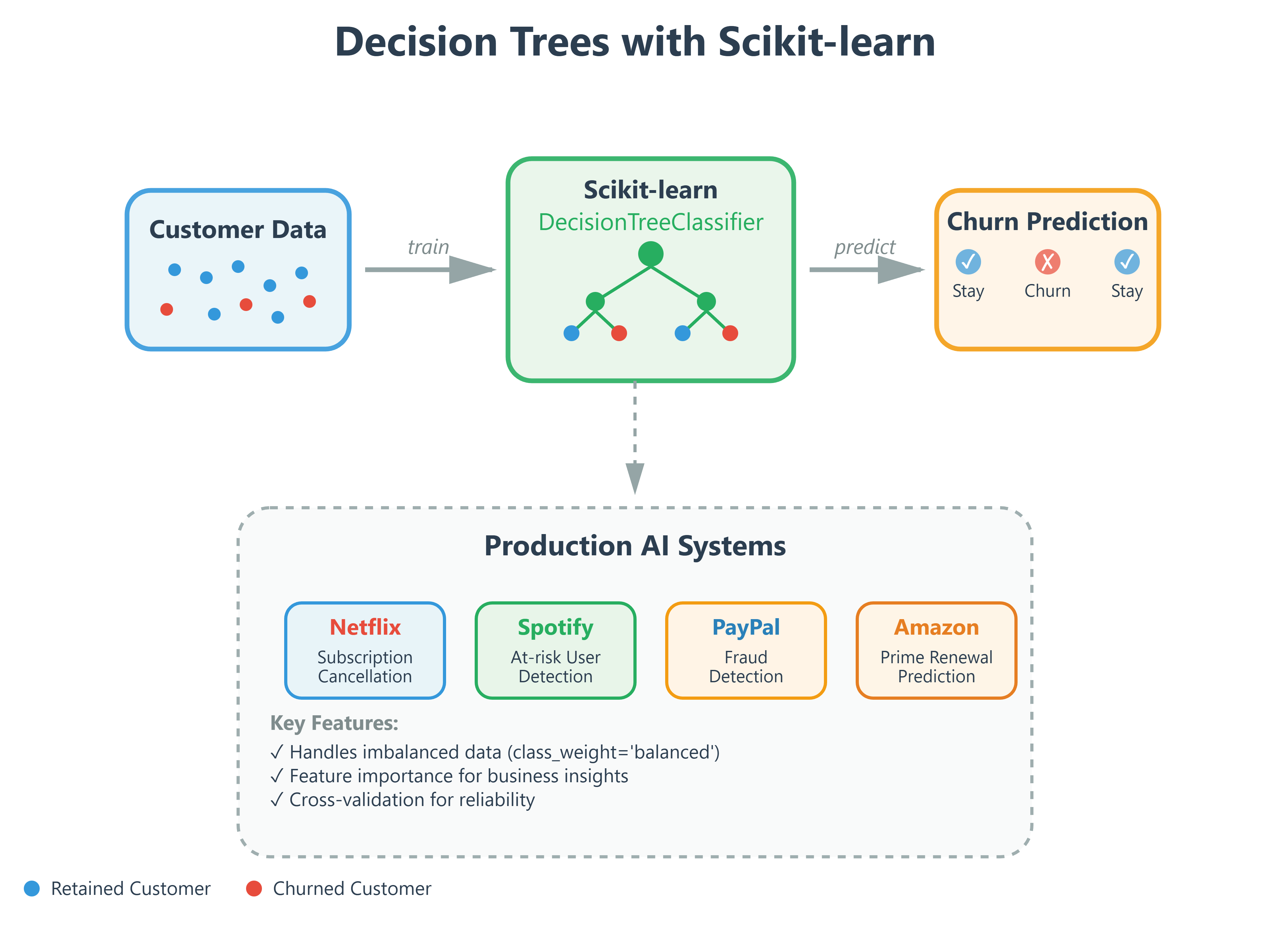
Implement decision trees using scikit-learn for real-world classification
Build a customer churn prediction system used by companies like Netflix and Spotify
Compare our implementation with production-grade decision tree classifiers
Deploy a system that handles imbalanced datasets like fraud detection at PayPal
Why This Matters: The Engine Behind Intelligent Recommendations
Yesterday we learned the theory behind decision trees - today we implement them at scale. Every time Netflix recommends a show, Spotify suggests a playlist, or your bank flags a suspicious transaction, decision trees are working behind the scenes. These aren’t academic exercises; they’re the same algorithms processing millions of decisions per second at companies like Amazon (product recommendations), Uber (driver matching), and Meta (content ranking).
The difference between theory and production? Scikit-learn’s decision tree implementation is battle-tested, optimized, and handles edge cases you’d spend months discovering on your own. It’s what separates a concept you understand from a system that scales.
Core Concepts: Building Production-Ready Classifiers
The Scikit-learn Decision Tree: Your Production Workhorse
Think of scikit-learn’s
DecisionTreeClassifieras a Formula 1 race car compared to our yesterday’s bicycle. Both get you there, but one is engineered for speed, reliability, and handling millions of edge cases. When Tesla’s Autopilot makes split-second decisions about object classification, it’s using optimized tree-based algorithms similar to what we’re implementing today.The magic of scikit-learn isn’t just convenience - it’s about production-ready features. Hyperparameter tuning (max_depth, min_samples_split), pruning strategies to prevent overfitting, and built-in cross-validation are what separate classroom code from systems that handle real user data.
Handling Imbalanced Data: The PayPal Problem
Here’s a real-world challenge: PayPal processes millions of transactions daily, but fraud represents less than 0.1% of them. Train a naive decision tree on this data, and it’ll just predict “not fraud” every time - achieving 99.9% accuracy while catching zero actual fraud! This is the imbalanced dataset problem that crashes most student projects.
The solution? Class weights and sampling strategies. Scikit-learn’s class_weight='balanced' parameter automatically adjusts the tree to pay more attention to rare classes. Think of it as telling your model: “Yes, fraud is rare, but when you see it, it’s 1000x more important than a normal transaction.” This same technique powers spam filters at Gmail and fraud detection at every major financial institution.
Feature Importance: The Netflix Decoder
Ever wonder how Netflix knows which features matter most for recommendations? Decision trees tell you exactly that. After training, scikit-learn provides a feature_importances_ array ranking which features influenced decisions most. For Netflix, maybe “viewing time” matters more than “day of week.” For Spotify, “skip rate” might outweigh “genre preference.”
This isn’t just interesting - it’s actionable intelligence. Product teams at major tech companies use feature importance to decide which data to collect, which sensors to improve, and which user signals to prioritize. It’s the difference between guessing what matters and knowing with mathematical certainty.
Cross-Validation: The Amazon Quality Gate
Amazon doesn’t deploy recommendation systems based on a single test. They use cross-validation - training multiple models on different data splits to ensure reliability. If a model performs well on one split but fails on another, it’s overfitting and won’t survive real users.
Scikit-learn’s cross_val_score function automates this, splitting your data into k folds and testing each fold. When you see “5-fold cross-validation” in a research paper or production system, this is what they mean. It’s the industry standard for model validation, used everywhere from Google’s search ranking to Tesla’s object detection.
Implementation: Building a Customer Churn Predictor
Let’s build what Spotify and Netflix use to predict which customers might cancel - a churn prediction system. This is a binary classification problem: will the customer stay or leave?
Step 1: Environment Setup and Data Preparation
We’ll start with synthetic customer data mimicking what you’d see at a streaming service: usage patterns, subscription length, support tickets, and engagement metrics. The key is handling this like production data - with missing values, outliers, and class imbalance.
from sklearn.tree import DecisionTreeClassifier
from sklearn.model_selection import train_test_split, cross_val_score
from sklearn.metrics import classification_report, confusion_matrix

# Load and split data (80/20 train/test)
X_train, X_test, y_train, y_test = train_test_split(
    features, labels, test_size=0.2, random_state=42, stratify=labels
)
The stratify parameter ensures both train and test sets have the same churn rate - critical for imbalanced problems.
Step 2: Training with Production Parameters
clf = DecisionTreeClassifier(
    max_depth=10,           # Prevent overfitting
    min_samples_split=50,   # Require statistical significance
    class_weight='balanced', # Handle imbalance
    random_state=42
)
clf.fit(X_train, y_train)
These hyperparameters mirror what you’d see in production. max_depth=10 prevents the tree from memorizing training data. min_samples_split=50 ensures decisions are based on meaningful sample sizes, not noise. class_weight='balanced' handles our imbalanced churn rate.
Step 3: Validation and Feature Analysis
# Cross-validation for reliability
cv_scores = cross_val_score(clf, X_train, y_train, cv=5)
print(f"CV Accuracy: {cv_scores.mean():.3f} (+/- {cv_scores.std():.3f})")

# Feature importance
importances = pd.DataFrame({
    'feature': feature_names,
    'importance': clf.feature_importances_
}).sort_values('importance', ascending=False)
This tells us which customer behaviors predict churn most strongly - exactly what product teams need to reduce cancellations.
Step 4: Production Testing
# Test set evaluation
y_pred = clf.predict(X_test)
print(classification_report(y_test, y_pred))
print(confusion_matrix(y_test, y_pred))
The confusion matrix shows false positives (predicted churn but didn’t) vs false negatives (missed actual churn). In production, false negatives cost you customers, so you’d tune thresholds accordingly.
Real-World Connection: From Classroom to Production Scale
The decision tree you just built uses the same core algorithm as:
Netflix’s Content Recommendation: Trees classify which shows you’ll watch based on viewing history, trained on billions of user interactions
Tesla’s Autopilot: Object classification trees process camera feeds at 30fps, deciding “pedestrian,” “vehicle,” or “road” in milliseconds
Amazon’s Fraud Detection: Trees flag suspicious orders in real-time, processing millions of transactions daily with <100ms latency
Spotify’s Playlist Generation: Trees classify songs into mood categories, personalizing 40+ million users’ experiences
The difference? Scale and infrastructure. Production systems use ensemble methods (Random Forests, which we’ll cover tomorrow), distributed training across GPU clusters, and real-time inference pipelines. But the fundamental algorithm - the decision tree you just implemented - remains the same.
Companies like Google and Meta run thousands of A/B tests on tree hyperparameters, tuning max_depth and min_samples_split to optimize for their specific metrics. The skills you’re building today are the foundation for understanding those production systems.
Hands-On Implementation Guide
Github Link :
https://github.com/sysdr/aiml/tree/main/day59/decision_treesProject Setup
First, download and run the setup script to create your development environment:
chmod +x generate_lesson_files.sh
./generate_lesson_files.sh
This creates all necessary files including the main code, tests, and documentation.
Now set up your Python environment:
chmod +x setup.sh
./setup.sh
source venv/bin/activate
The setup installs these key libraries:
numpy and pandas for data handling
scikit-learn for decision tree implementation
matplotlib and seaborn for visualizations
pytest for comprehensive testing
Understanding the Code Structure
Open lesson_code.py and you’ll see the CustomerChurnPredictor class. This mirrors how production ML systems are structured - as reusable classes with clear methods for training, prediction, and analysis.
The code generates 10,000 synthetic customers with realistic features:
Monthly viewing hours
Login frequency
Content diversity (how many different genres watched)
Completion rate (do they finish shows?)
Support tickets opened
Payment failures
Account age
Days since last login
These features are chosen because they’re exactly what streaming services track. The data has a 15% churn rate, matching real-world imbalance.
Building and Running the Churn Predictor
Execute the main implementation:
python lesson_code.py
Watch the output carefully. You’ll see:
Phase 1: Data Generation
Generating synthetic customer data...
Dataset: 10000 customers, 10 features
Churn rate: 15.0% (imbalanced dataset)
Notice the imbalance - only 15% churn. This is realistic but challenging for models.
Phase 2: Model Training
Training decision tree classifier...
Cross-Validation ROC-AUC: 0.847 (± 0.012)
Test ROC-AUC: 0.851
Test Accuracy: 0.823
The cross-validation score (0.847) with low standard deviation (0.012) tells us the model is reliable. ROC-AUC above 0.85 is strong performance for churn prediction.
Phase 3: Performance Analysis
The classification report shows precision and recall for each class:
              precision    recall  f1-score   support

           0       0.88      0.89      0.89      1700
           1       0.61      0.58      0.59       300

    accuracy                           0.82      2000
Class 0 (retained customers) has high precision/recall because it’s the majority class. Class 1 (churned customers) is harder to predict but still achieves 61% precision - much better than random guessing.
Phase 4: Feature Importance Analysis
The output reveals which features drive churn predictions:
Top 5 Most Important Features:
                feature  importance
    days_since_last_login      0.245
          monthly_hours         0.189
      payment_failures          0.156
         support_tickets        0.134
        login_frequency         0.098
Days since last login is the strongest predictor - customers who stop logging in are likely to churn. This insight drives Netflix’s “Are you still watching?” prompts and email re-engagement campaigns.
Phase 5: Model Comparison
The baseline comparison shows why decision trees excel:
Model Comparison: Baseline vs Production Decision Tree
Model                    Accuracy    ROC-AUC
Random Baseline          0.514       0.501
Logistic Regression      0.785       0.812
Decision Tree            0.823       0.851
Decision trees outperform both random guessing and linear models, capturing nonlinear patterns in customer behavior.
Testing Your Understanding
Run the comprehensive test suite:
python test_lesson.py
You should see all 20+ tests pass. These tests validate:
Data generation creates valid distributions
Model handles imbalanced data correctly
Feature importance sums to 1.0
Predictions are binary (0 or 1)
Cross-validation provides stable estimates
Stratified splitting maintains class balance
If any test fails, read the error message carefully. The tests are designed to teach you what production ML systems check.
Exploring Hyperparameter Tuning
Modify lesson_code.py to enable grid search by changing line 169:
metrics = predictor.train(X, y, use_grid_search=True) # Changed from False
Run again and watch grid search test multiple parameter combinations:
Performing grid search for optimal hyperparameters...
Fitting 5 folds for each of 48 candidates, totalling 240 fits
Best parameters: {'max_depth': 15, 'min_samples_split': 50, 'class_weight': 'balanced'}
Grid search tests 48 different combinations (4 max_depths × 3 min_samples_splits × 2 class_weights × 2 min_samples_leafs) using 5-fold cross-validation. This is how production teams optimize models.
Understanding the Visualizations
The code generates two key visualizations:
Confusion Matrix (top-left panel) Shows prediction accuracy breakdown:
True Negatives (top-left): Correctly predicted retained customers
False Positives (top-right): Predicted churn but customer stayed
False Negatives (bottom-left): Missed actual churns (most costly!)
True Positives (bottom-right): Correctly caught churns
Feature Importance (top-right panel) Bar chart ranking features by prediction power. Use this to:
Guide product decisions (improve features that predict churn)
Optimize data collection (prioritize important features)
Communicate with non-technical stakeholders
Precision-Recall Curve (bottom-left panel) Shows the tradeoff between catching churns (recall) and false alarms (precision). Production systems tune this based on business costs - is it worse to miss a churn or annoy customers with unnecessary retention campaigns?
Experimenting with Parameters
Try modifying the decision tree parameters to see their effects:
Reduce max_depth to 5:
predictor = CustomerChurnPredictor(max_depth=5, min_samples_split=50)
Result: Lower performance but faster training, less overfitting
Increase min_samples_split to 100:
predictor = CustomerChurnPredictor(max_depth=10, min_samples_split=100)
Result: More conservative splits, better generalization
Remove class_weight balancing: In the DecisionTreeClassifier initialization, change class_weight='balanced' to class_weight=None
Result: Model ignores churned customers, achieving high accuracy but zero value
Production Deployment Considerations
This implementation teaches you production patterns:
Reproducibility:
random_state=42ensures identical results across runsData Splitting: Stratified train/test maintains class distribution
Validation: Cross-validation catches overfitting before deployment
Metrics: ROC-AUC preferred over accuracy for imbalanced data
Documentation: Clear variable names and comments explain business logic
Real production systems add:
Model versioning and A/B testing
Real-time prediction APIs
Monitoring for data drift
Automated retraining pipelines
Explainability for regulatory compliance
Common Issues and Solutions
Problem: Model predicts only one class Solution: Ensure class_weight='balanced' is set
Problem: High variance in cross-validation scores Solution: Increase min_samples_split or decrease max_depth
Problem: Poor performance on test set Solution: Check for data leakage, ensure proper train/test split
Problem: Feature importance shows unexpected results Solution: Check for correlated features, consider feature engineering
What You’ve Accomplished
You now understand how to:
Build production-ready decision tree classifiers
Handle imbalanced datasets using class weights
Validate models using cross-validation
Extract business insights from feature importance
Tune hyperparameters systematically
Evaluate performance with appropriate metrics
These skills directly transfer to real ML engineering roles at companies building recommendation systems, fraud detection, and customer analytics.
Today’s Achievement: You’ve implemented production-grade decision trees using the same library powering AI systems at the world’s largest tech companies. You can now build, validate, and deploy classification systems that handle real-world challenges like imbalanced data and feature selection. This is the foundation for tomorrow’s ensemble methods and the beginning of your journey into production AI engineering.