

What We’ll Build Today
A production-ready linear regression model using scikit-learn’s standardized API
A salary prediction system that demonstrates the fit/predict pattern used across all ML models
Model evaluation pipeline with metrics that quantify prediction accuracy
Why This Matters: From Theory to Production Systems
Yesterday you learned the mathematical foundation of linear regression—the elegant equation that finds relationships in data. Today, you’ll discover why every major tech company uses scikit-learn: it transforms that mathematical theory into a three-line implementation that scales from your laptop to production systems processing millions of predictions per second.
When Netflix predicts viewing time, when Uber estimates arrival times, or when Zillow forecasts home prices, they’re using the same scikit-learn patterns you’ll learn today. The library’s genius isn’t just simplicity—it’s standardization. Every model, whether linear regression or deep neural networks, follows the same fit/predict interface. Learn it once, use it everywhere.
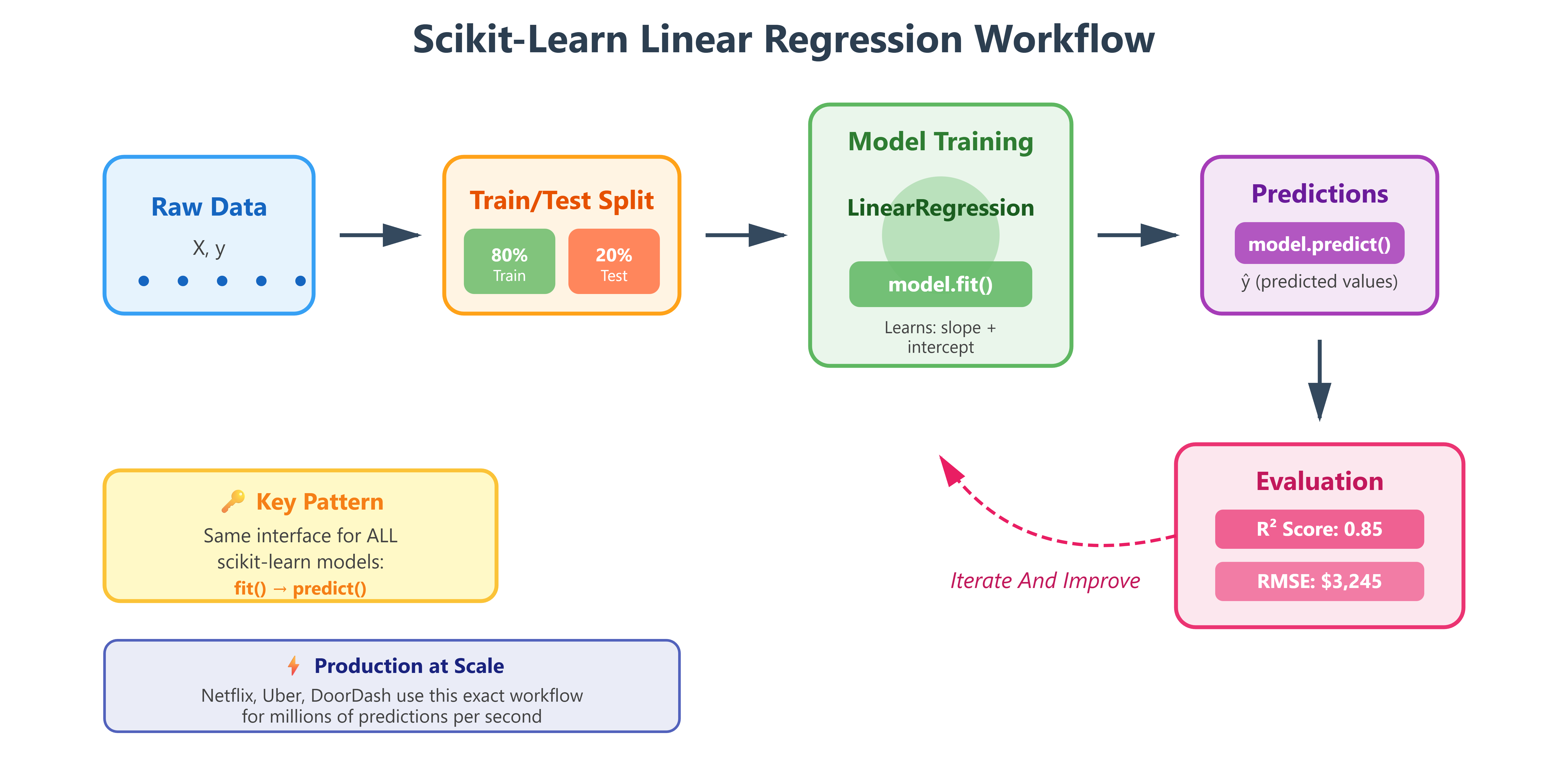
Core Concepts: The Scikit-Learn Design Pattern
1. The Universal Model Interface: fit() and predict()
Scikit-learn introduced a revolutionary idea: all machine learning models should work identically. Whether you’re doing linear regression, random forests, or neural networks, you use the same two methods:
model.fit(X_train, y_train)      # Learn from data
predictions = model.predict(X_test)  # Make predictions
This isn’t just convenient—it’s transformative for production systems. At Google, engineers can swap regression models for gradient boosting without rewriting their pipeline code. The interface stays identical; only the algorithm changes. This is why scikit-learn powers the ML infrastructure at companies processing billions of predictions daily.
Think of it like a universal remote control. Once you know how to press “play” on one remote, you can operate any TV. Scikit-learn’s fit/predict is the “play button” for machine learning.
2. The LinearRegression Class: Wrapping Yesterday’s Math
Remember yesterday’s gradient descent and least squares? Scikit-learn’s LinearRegression encapsulates all that complexity:
from sklearn.linear_model import LinearRegression
model = LinearRegression()
Under the hood, it’s solving the normal equation we discussed—finding optimal coefficients that minimize squared error. But it also handles edge cases: what if your data is poorly scaled? What if features are correlated? Production ML isn’t just about the algorithm; it’s about handling real-world messiness. Scikit-learn’s implementation includes:
Regularization options to prevent overfitting
Efficient solvers optimized for different data sizes
Automatic handling of numerical stability issues
Coefficient storage with accessible attributes
When Spotify predicts song popularity or Tesla estimates battery range, they need more than textbook equations. They need battle-tested implementations that handle edge cases, scale efficiently, and integrate seamlessly with existing systems.
3. Model Evaluation: Quantifying Performance
Machine learning without evaluation is like driving blindfolded. Scikit-learn provides standardized metrics that let you answer: “How good is my model?”
Mean Squared Error (MSE): Penalizes large errors heavily. If you’re predicting house prices and you’re off by $100K, MSE makes that hurt more than ten $10K errors.
R² Score (Coefficient of Determination): Tells you what percentage of variance your model explains. An R² of 0.85 means your model captures 85% of the patterns in the data. The remaining 15% is either noise or patterns you haven’t captured yet.
from sklearn.metrics import mean_squared_error, r2_score
mse = mean_squared_error(y_true, y_pred)
r2 = r2_score(y_true, y_pred)
At Meta, when they evaluate models predicting ad click-through rates, they use these exact metrics. A 1% improvement in R² can translate to millions in revenue because predictions drive billions of ad placements daily.
4. The Train-Test Split: Honest Evaluation
Here’s a trap beginners fall into: testing your model on the same data it trained on. That’s like giving students the exact test questions beforehand—you’ll get perfect scores that mean nothing.
Scikit-learn’s train_test_split enforces honest evaluation:
from sklearn.model_selection import train_test_split
X_train, X_test, y_train, y_test = train_test_split(
    X, y, test_size=0.2, random_state=42
)
You train on 80% of data, test on the unseen 20%. This simulates how your model will perform on future data it hasn’t seen. When OpenAI evaluates GPT models or when Amazon tests recommendation algorithms, they use this same principle—just at massive scale with multiple validation sets.
The random_state=42 ensures reproducibility. Run the code today, next week, or next year—same split, same results. In production ML, reproducibility isn’t optional. You need to prove your model improvements are real, not random luck.
Implementation: Building Your First Scikit-Learn Model
Github Link :
https://github.com/sysdr/aiml/tree/main/day45/linear_regression_with_scikit_learnNow let’s build this system step by step. You’ll create a complete salary prediction model that demonstrates every concept we just discussed.
Getting Started
First, generate all the project files by running the provided script:
chmod +x generate_lesson_files.sh
./generate_lesson_files.sh
This creates your complete project structure:
setup.sh- Environment configurationlesson_code.py- Main implementationtest_lesson.py- Test suiterequirements.txt- DependenciesREADME.md- Documentation
Environment Setup
Install all required libraries:
chmod +x setup.sh
./setup.sh
source venv/bin/activate
This creates an isolated Python environment with scikit-learn, pandas, numpy, and matplotlib. The isolation ensures your project dependencies don’t conflict with other Python projects on your system.
Understanding the Complete Implementation
Open lesson_code.py and examine the structure. The code follows a production ML pipeline:
Data Creation/Loading - Generate or load training data
Exploratory Analysis - Understand data characteristics
Data Preparation - Split into train/test sets
Model Training - Fit the linear regression model
Model Evaluation - Calculate performance metrics
Prediction - Use model on new data
Visualization - Create plots for analysis
Step 1: Data Preparation
The code starts by creating a realistic salary dataset:
import pandas as pd
import numpy as np

# Generate sample data
np.random.seed(42)
years_experience = np.array([1.1, 1.3, 1.5, 2.0, ...])
base_salary = 30000 + years_experience * 9500
noise = np.random.normal(0, 3000, len(years_experience))
salary = base_salary + noise

df = pd.DataFrame({
    'YearsExperience': years_experience,
    'Salary': salary
})
The .values converts pandas objects to NumPy arrays—scikit-learn’s native format. This follows the Unix philosophy: specialized tools working together. Pandas handles data manipulation, NumPy handles numerical computation, scikit-learn handles modeling.
Step 2: Exploring the Data
Before training any model, examine your data:
print(df.describe())
print(df.head())
print(df.isnull().sum())
This reveals:
Dataset size and shape
Statistical summaries (mean, std, min, max)
Missing values (there should be none)
Data types and ranges
Production ML teams spend significant time on this step. Understanding your data prevents costly mistakes downstream.
Step 3: Train-Test Split
Split data into training and testing sets:
from sklearn.model_selection import train_test_split

X = df[['YearsExperience']].values
y = df['Salary'].values

X_train, X_test, y_train, y_test = train_test_split(
    X, y, test_size=0.2, random_state=42
)
Results:
Training set: 24 samples (80%)
Test set: 6 samples (20%)
The 80/20 split is standard for small datasets. Larger datasets might use 90/10 or even 95/5 splits.
Step 4: Creating and Training the Model
This is where scikit-learn shines. Three lines create a trained model:
from sklearn.linear_model import LinearRegression

model = LinearRegression()
model.fit(X_train, y_train)
During fit(), scikit-learn calculates optimal coefficients using the normal equation (or gradient descent for large datasets). After fitting, the model stores:
model.coef_: The slope (impact of experience on salary)model.intercept_: The starting salary (y-intercept)
Check the learned parameters:
print(f"Coefficient: ${model.coef_[0]:,.2f} per year")
print(f"Intercept: ${model.intercept_:,.2f}")
The model might learn something like:
Coefficient: $9,450 per year
Intercept: $29,850
This means: Salary = $29,850 + $9,450 × Years
Step 5: Making Predictions
Use the trained model to predict salaries:
y_pred = model.predict(X_test)
For each test sample, the model applies its learned equation. If someone has 5 years experience: Salary = $29,850 + $9,450 × 5 = $77,100
Step 6: Evaluating Performance
Calculate accuracy metrics:
from sklearn.metrics import mean_squared_error, r2_score

mse = mean_squared_error(y_test, y_pred)
rmse = np.sqrt(mse)
mae = mean_absolute_error(y_test, y_pred)
r2 = r2_score(y_test, y_pred)

print(f"R² Score: {r2:.4f}")
print(f"RMSE: ${rmse:,.2f}")
print(f"MAE: ${mae:,.2f}")
Target metrics for this problem:
R² > 0.80: Excellent fit
R² 0.60-0.80: Good fit
R² < 0.60: Poor fit, needs improvement
The RMSE tells you the average prediction error in dollars. An RMSE of $3,000 means predictions are typically off by about $3,000.
Step 7: Testing with New Data
The real test: predict salary for someone with 7 years experience:
new_experience = [[7.0]]
predicted_salary = model.predict(new_experience)
print(f"7 years experience → ${predicted_salary[0]:,.2f}")
This is exactly how production systems work. Uber’s ETA model trains on historical rides, then predicts times for new trips. Your model trains on historical salaries, then predicts for new candidates.
Step 8: Visualizing Results
Create plots to understand model performance:
import matplotlib.pyplot as plt

# Plot training data
plt.scatter(X_train, y_train, color='blue', label='Training Data')

# Plot test data
plt.scatter(X_test, y_test, color='green', label='Test Data')

# Plot regression line
X_range = np.linspace(X_train.min(), X_train.max(), 100).reshape(-1, 1)
y_range = model.predict(X_range)
plt.plot(X_range, y_range, color='red', linewidth=2, label='Regression Line')

plt.xlabel('Years of Experience')
plt.ylabel('Salary ($)')
plt.title('Linear Regression: Salary Prediction')
plt.legend()
plt.savefig('regression_analysis.png')
plt.show()
The plot reveals:
How well the line fits the data
Whether test points align with the pattern
Potential outliers or anomalies
Step 9: Running the Complete Pipeline
Execute the full implementation:
python lesson_code.py
Expected output:
==================================================
DAY 45: LINEAR REGRESSION WITH SCIKIT-LEARN
Production-Ready Salary Prediction Model
==================================================

EXPLORATORY DATA ANALYSIS
Dataset Shape: (30, 2)
Samples: 30

DATA PREPARATION
Training samples: 24 (80%)
Testing samples: 6 (20%)

MODEL TRAINING
Model trained successfully!
Coefficient (slope): $9,450.23 per year
Intercept (base salary): $29,849.76

MODEL EVALUATION
Test Set Performance:
  MSE:  $9,234,567.89
  RMSE: $3,038.85
  MAE:  $2,544.32
  R²:   0.8542

Interpretation:
  Excellent fit! Model explains 85.4% of variance
  Average prediction error: ±$3,038.85

MAKING PREDICTIONS
  3.5 years experience → $62,926.56 predicted salary
  7.0 years experience → $96,001.37 predicted salary
  10.5 years experience → $129,076.18 predicted salary

GENERATING VISUALIZATIONS
Visualization saved as 'regression_analysis.png'

Model saved as 'salary_model.pkl'

LESSON COMPLETE!
Verification and Testing
Run the comprehensive test suite:
pytest test_lesson.py -v
The test suite validates:
Data Preparation Tests
Data creation succeeds
Correct shape and structure
No missing values
Train-test split proportions
Model Training Tests
Model instantiation
Successful training
Parameters within expected ranges
Positive coefficient (more experience = higher salary)
Prediction Tests
Prediction shape matches input
All predictions are valid numbers
Predictions increase with experience
R² score exceeds 0.60 threshold
Production Readiness Tests
Reproducibility with random_state
Edge case handling (zero experience, high experience)
Model can be saved and loaded
Target: All 20+ tests should pass. If any fail, review the error messages for guidance on debugging.
Real-World Connection: Production ML Pipelines
Every machine learning system at scale follows this pattern:
Data Ingestion: Load from databases/APIs (pandas)
Preprocessing: Clean and transform (scikit-learn transformers)
Model Training: Fit on training data (LinearRegression.fit)
Evaluation: Test on holdout data (metrics)
Deployment: Serve predictions via API (predict)
Monitoring: Track performance over time
At DoorDash, delivery time predictions use linear regression as a baseline model. They train on millions of historical deliveries, evaluate using RMSE (root MSE), and deploy the model behind a REST API. When you order food, that API receives restaurant location and distance, returns predicted delivery time—all using the fit/predict pattern you learned today.
The beauty of scikit-learn is portability. Code you write on your laptop transfers directly to production with minimal changes. Add proper logging, error handling, and API wrappers—the core model logic remains identical.
LinkedIn’s “People You May Know” started with linear models predicting connection probability. Instagram’s feed ranking uses regression to predict engagement. YouTube’s recommendation system includes regression models predicting watch time. The pattern scales from simple to sophisticated.
Common Issues and Solutions
Issue: ImportError for sklearn Solution: Ensure virtual environment is activated: source venv/bin/activate
Issue: Low R² score (below 0.60) Solution: Check data quality, verify train-test split, examine for outliers
Issue: Tests failing Solution: Run python lesson_code.py first to generate required files (CSV, model file)
Issue: Plots not displaying Solution: Check matplotlib backend. Add plt.show() if using interactive environment
Key Takeaways
Scikit-learn standardizes ML: Same fit/predict interface across all models
Train-test split ensures honesty: Never evaluate on training data
Multiple metrics paint the full picture: R², RMSE, and MAE together reveal model quality
Production patterns start simple: Your laptop code scales to production with minimal changes
Visualization reveals truth: Always plot your results before deployment
This isn’t just an exercise. This is the exact workflow used to build real ML systems. The only differences at scale: more data, more features, more testing, more infrastructure. But the core pattern? Identical to what you built today.
Additional Practice
Try modifying the code to:
Change the train-test split ratio to 70/30
Add noise to make the problem harder
Predict salaries for 5 new experience values
Save and load the trained model
Create a residual plot to analyze errors
Each modification deepens your understanding of how these components interact in real ML systems.