What We Are Building Today
By the end of this lesson you will have done three things that actually matter:
Understood why sequential data breaks standard networks — and what RNNs do differently at the architectural level.
Decoded how LSTMs solve the vanishing gradient problem that crippled early RNNs, using three learned memory gates.
Built a working character-level language model that generates text one character at a time — the same core idea behind every autocomplete you have ever used.
Connected this to production systems at Google, Amazon, Apple, and Stripe that run LSTM-based models today.
Why This Matters
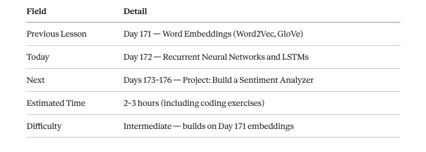
Yesterday you built word embeddings — dense vector representations of meaning. Today you learn how to process sequences of those vectors over time. Every autocomplete suggestion you have typed, every translation you have read, every voice command your phone understood — all of it traces back to the sequential modeling ideas you will master today.
Even in the age of transformers, understanding RNNs and LSTMs is not optional. Production systems at Apple (on-device Siri models), Amazon (Alexa keyword detection), and trading firms (time-series forecasting) still run LSTM-based models because they are computationally lighter and interpretable. Knowing why transformers replaced RNNs requires understanding what RNNs got wrong. That knowledge gap is what separates engineers who implement AI from engineers who design it.
Core Concepts
1. The Sequence Problem — Why Feedforward Networks Fall Short
A standard dense neural network treats every input as independent. Feed it “The cat sat on the ___” and it sees seven unrelated word vectors with no awareness of order. The network has no memory — it cannot know that “cat” modifies what comes after “sat.”
Think of it like reading a book where each page is shuffled randomly. You see the words, but the story is gone.
RNNs fix this by introducing a hidden state — a memory vector that gets updated at every time step. At step
t, the network takes two inputs: the current word vectorx_tand the hidden state from the previous steph_{t-1}. The output hidden stateh_tencodes everything the network has seen up to positiont.
h_t = tanh( W_hh · h_{t-1} + W_xh · x_t + b )
That shared weight matrix W_hh is identical at every time step — it is what makes RNNs parameter-efficient. A 10-step sequence and a 1,000-step sequence use exactly the same parameter count.
2. The Vanishing Gradient — The RNN’s Achilles Heel
Here is the bitter irony. Backpropagation through an RNN means multiplying gradients across every time step. If those gradients are smaller than 1.0 (which they almost always are after a tanh), they shrink exponentially. By the time you are 50 steps back, the gradient is effectively zero.
The network literally forgets what happened earlier in the sequence. Training an RNN on a long paragraph and asking it to remember the subject from sentence one is like whispering a secret across 100 people — by the end, the message is noise.
Key Insight — The Vanishing Gradient Problem This is the single biggest reason vanilla RNNs struggle with dependencies longer than roughly 10–20 tokens. Each time step multiplies gradients together, and repeated multiplication of values less than 1.0 sends them toward zero exponentially fast. LSTMs were invented specifically to fix this.
3. LSTMs — Learned Memory Management
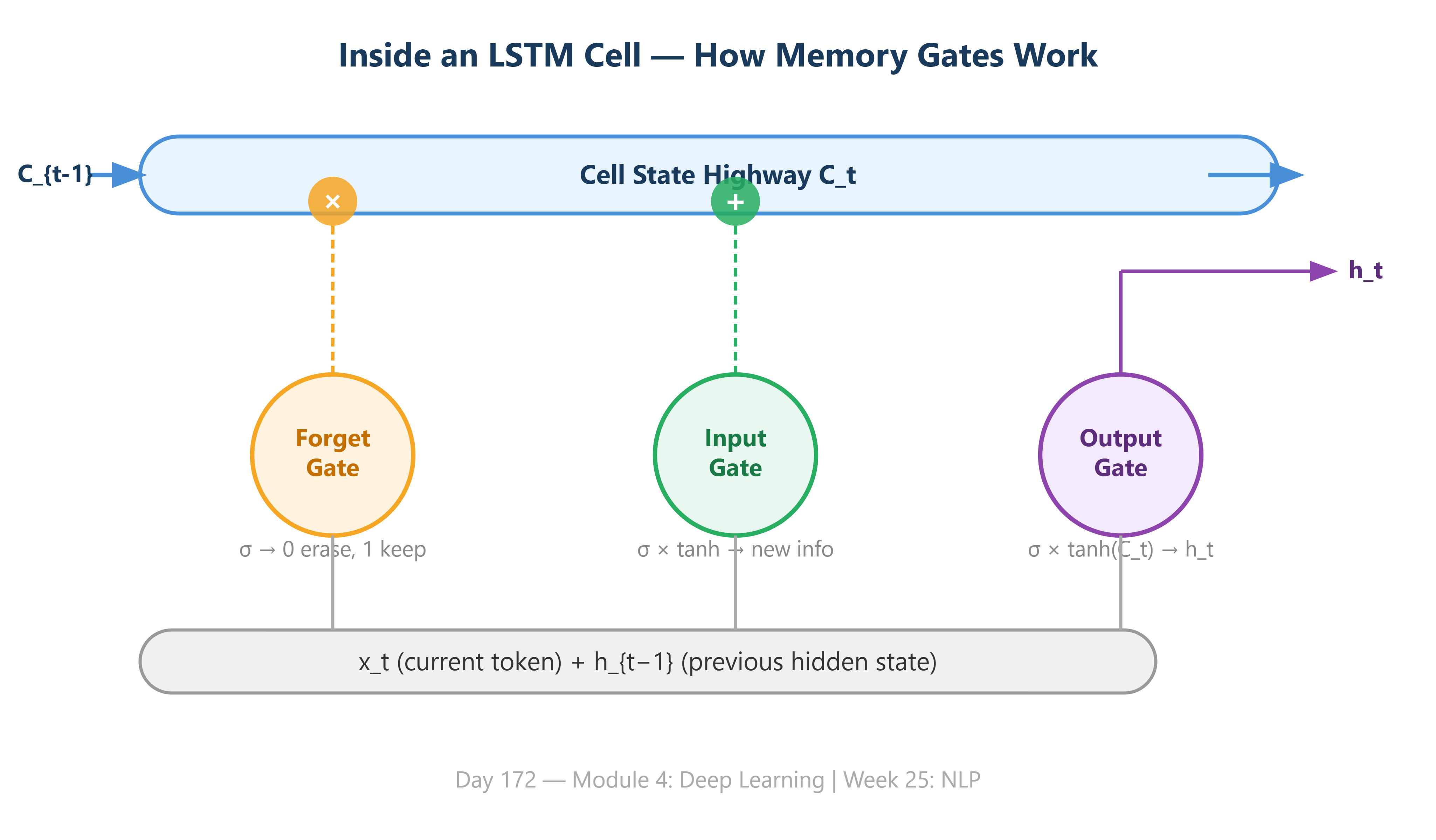
Long Short-Term Memory networks (Hochreiter & Schmidhuber, 1997) solve the vanishing gradient problem with a second memory channel: the cell state C_t. Where the hidden state is your working memory, the cell state is long-term storage — and crucially, information flows through it additively, not multiplicatively.
LSTMs use three learned gates to control information flow: