

Today’s Agenda
What computer vision actually is, and why it matters beyond “image recognition”
How raw pixels become structured data that neural networks can learn from
The classic CV pipeline: acquire, preprocess, extract, classify
Hands-on: build an image preprocessing pipeline using OpenCV and PIL
How production CV systems at Google, Tesla, and Waymo handle millions of frames per second
Why This Matters
You have spent the last 28 days building neural networks that work on numbers in tables. Computer vision breaks that constraint entirely. The moment you can teach a model to understand images, you unlock a class of problems that touches nearly every industry on the planet: autonomous vehicles reading road signs, radiologists’ assistants flagging tumors in X-rays, warehouse robots locating items on shelves, retail systems tracking inventory without barcodes.
Every one of those systems starts with the same foundational step you are learning today: turning a raw image into a tensor a neural network can process. This is the bridge between the physical world and the computational one.
Core Concepts
What an Image Actually Is
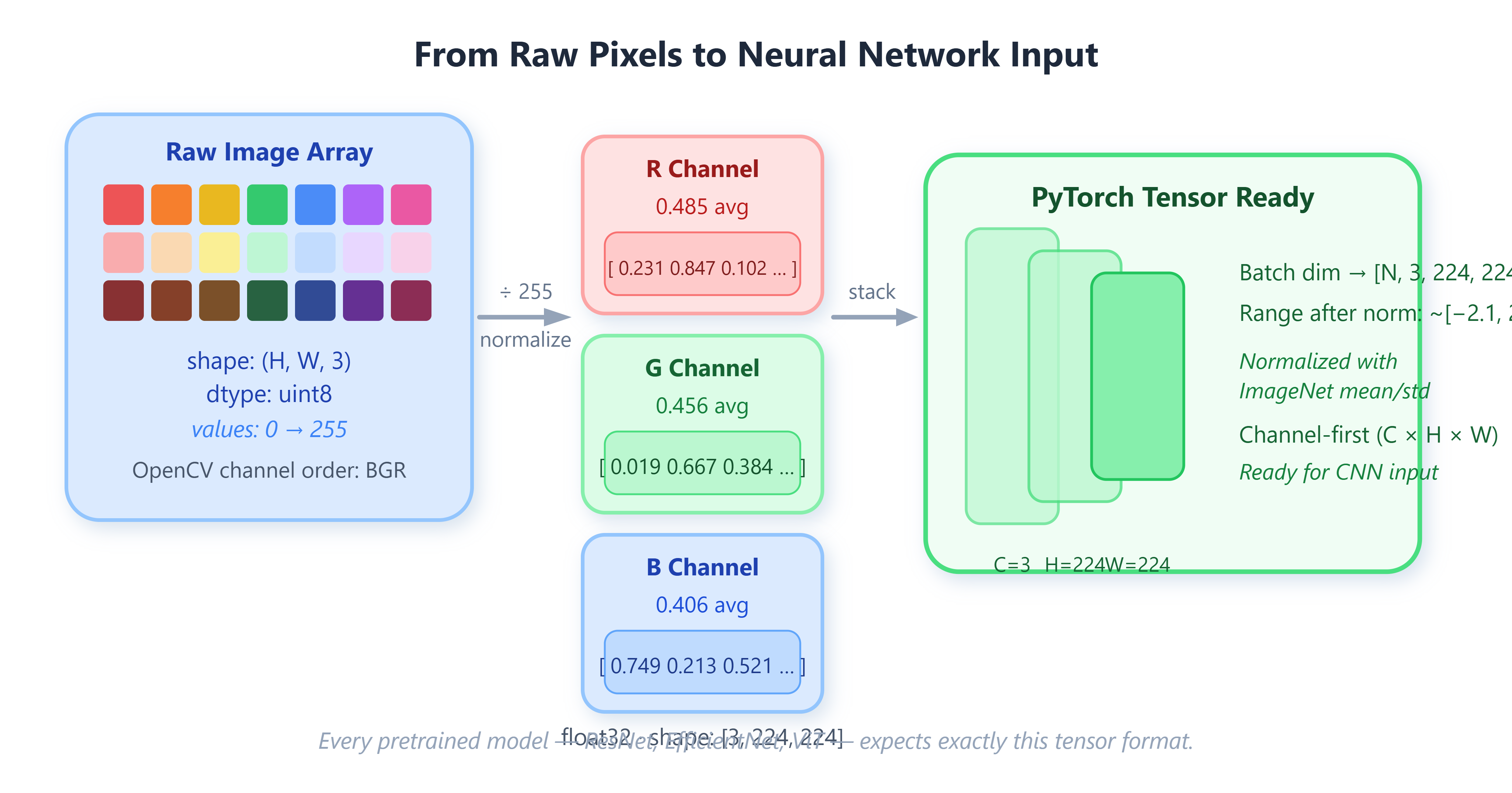
An image is nothing more than a 3-dimensional array of numbers. A standard color photo with dimensions 224 × 224 pixels is a tensor of shape (224, 224, 3), where the three channels represent red, green, and blue intensity values ranging from 0 to 255. Grayscale images collapse to (224, 224, 1). That is it. The moment you accept that an image is just a matrix of integers, the entire field of computer vision becomes approachable.
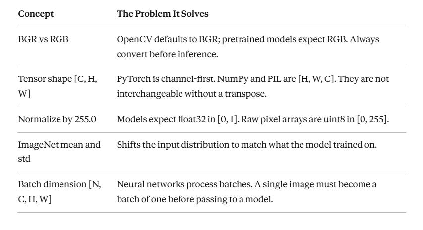
NumPy stores this as a uint8 array. PyTorch and TensorFlow expect float32 tensors with values normalized to the range [0.0, 1.0]. Every preprocessing pipeline you write will include a division by 255.0 at some point. That single operation is the handshake between the imaging world and the deep learning world.
The Four-Stage CV Pipeline
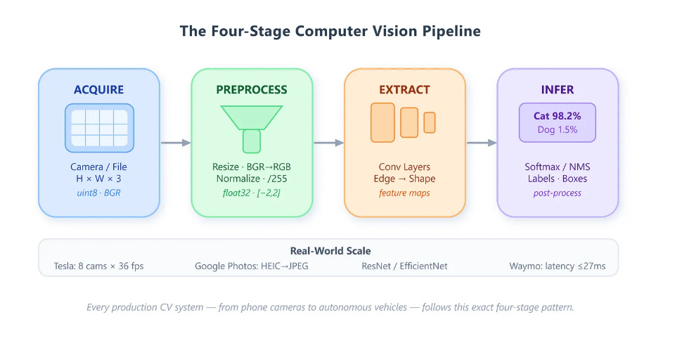
Production computer vision systems, from Google Lens to Tesla Autopilot, follow a consistent architecture regardless of their ultimate task.
Stage 1 — Acquisition. Raw image data enters the system from a camera, file system, or network stream. Resolution, color space, and frame rate are properties of the acquisition layer. Tesla’s FSD cameras capture at 36 frames per second across eight cameras simultaneously. Every frame must enter the pipeline within 27 milliseconds to maintain real-time performance.
Stage 2 — Preprocessing. Raw images are noisy, inconsistently sized, and poorly lit. Preprocessing normalizes all of that. Resizing to a fixed resolution (commonly 224 × 224 for ImageNet-pretrained models), converting color spaces (BGR to RGB is a classic OpenCV gotcha), applying normalization using dataset-specific mean and standard deviation values — these operations create the clean, consistent input tensors that models expect. Skipping or misapplying preprocessing is the single most common cause of poor model performance on good data.
Stage 3 — Feature Extraction. This is where neural networks replaced decades of hand-crafted algorithms. Before deep learning, engineers spent careers writing code to detect edges with Sobel filters, find corners with Harris detectors, and describe local patches with SIFT descriptors. Convolutional Neural Networks, which you will build tomorrow, learn those detectors automatically from data. Today, understanding that features are the intermediate representations of meaningful visual structure — edges, textures, shapes, objects — is the conceptual foundation you need.
Stage 4 — Inference and Post-processing. The model produces raw scores (logits) or bounding box coordinates. Post-processing converts those into human-readable outputs: class labels, confidence scores, pixel masks. Non-Maximum Suppression (NMS) for object detection, sigmoid/softmax for classification, and morphological operations for segmentation all live here.
Color Spaces and Channel Ordering
A persistent source of bugs in CV pipelines is channel ordering. OpenCV loads images in BGR order by default. PyTorch models trained on ImageNet expect RGB. Loading an image with cv2.imread() and passing it directly to a pretrained model produces subtly wrong results that are difficult to diagnose because the model still produces predictions, just worse ones. Always apply cv2.cvtColor(img, cv2.COLOR_BGR2RGB) when bridging OpenCV and PyTorch.
Watch out for this one. BGR vs RGB is the most common silent bug in new CV pipelines. The model will still run and produce predictions — they will just be quietly wrong. It is the kind of error that costs days of debugging. One line of code prevents it entirely.
Normalization: Mean and Standard Deviation
ImageNet-pretrained models expect inputs normalized with specific statistics: mean = [0.485, 0.456, 0.406] and std = [0.229, 0.224, 0.225] across the RGB channels. These numbers represent the channel-wise mean and standard deviation of the entire ImageNet training set. Applying this normalization ensures your input distribution matches what the model learned on. Forgetting this step when using pretrained weights is another quiet killer of model performance.
Why these specific numbers? They were computed once across all 1.2 million images in the ImageNet dataset and published with the original models. Every researcher and engineer in the field uses the same values. You will have them memorized by the end of this module.
Key Concepts at a Glance
Implementation
These five steps walk you through the full preprocessing pipeline from raw file to normalized tensor. The code is intentionally minimal — you are learning what each operation does before you run the full package.
1. Install the dependencies
pip install opencv-python-headless Pillow torch torchvision numpy matplotlib
2. Load and inspect a raw image
This is the acquisition stage. You are reading the file, confirming its shape, and understanding the data type before touching anything.
import cv2
import numpy as np
from PIL import Image

img_bgr = cv2.imread("sample.jpg")
print(f"Shape: {img_bgr.shape}")   # (H, W, 3)
print(f"Dtype: {img_bgr.dtype}")   # uint8
print(f"Range: [{img_bgr.min()}, {img_bgr.max()}]")
3. Build the preprocessing pipeline
transforms.Compose chains operations in order. ToTensor handles the /255.0 conversion and the HxWxC to CxHxW transpose simultaneously. Normalize applies the ImageNet statistics channel by channel.
import torch
from torchvision import transforms

preprocess = transforms.Compose([
    transforms.Resize((224, 224)),
    transforms.ToTensor(),                # uint8 HxWxC -> float32 CxHxW, divides by 255
    transforms.Normalize(
        mean=[0.485, 0.456, 0.406],
        std=[0.229, 0.224, 0.225]
    )
])

img_rgb = cv2.cvtColor(img_bgr, cv2.COLOR_BGR2RGB)
pil_img = Image.fromarray(img_rgb)
tensor  = preprocess(pil_img)
print(f"Tensor shape: {tensor.shape}")   # torch.Size([3, 224, 224])
print(f"Tensor range: [{tensor.min():.3f}, {tensor.max():.3f}]")
4. Batch multiple images
Models do not process a single image at a time — they process batches. torch.stack adds the N dimension, turning a list of [3, 224, 224] tensors into a single [N, 3, 224, 224] tensor ready for a model.
batch = torch.stack([preprocess(Image.open(p).convert("RGB")) for p in image_paths])
print(f"Batch shape: {batch.shape}")  # [N, 3, 224, 224]
5. Visualize preprocessed tensors
You cannot display a normalized tensor directly — the values are outside the 0–1 range that image viewers expect. This function reverses the normalization so you can confirm the preprocessing visually.
def tensor_to_displayable(tensor):
    # Undo normalization for visualization
    mean = torch.tensor([0.485, 0.456, 0.406]).view(3, 1, 1)
    std  = torch.tensor([0.229, 0.224, 0.225]).view(3, 1, 1)
    img  = tensor * std + mean
    img  = img.permute(1, 2, 0).numpy()
    return (img * 255).astype(np.uint8)
Build, Test, and Demo
Github Link:
https://github.com/sysdr/aiml/tree/main/day155/day155_cv_intro
The bash script scaffolds the full implementation package — lesson_code.py, test_lesson.py, setup.sh, requirements.txt, and README.md.
1. Run the demo
python lesson_code.py
Expected output:
=== Stage 1: Acquisition & Inspection ===
  shape_hwc: (100, 280, 3)
  dtype: uint8    pixel_min: 0    pixel_max: 255

=== Stage 2: Preprocessing ===
  Output tensor shape : torch.Size([3, 224, 224])
  Output tensor dtype : torch.float32

=== Stage 3: Channel Statistics ===
  R -> mean=-0.1823  std=1.0241  range=[-2.117, 2.640]
  G -> mean=-0.0514  std=0.9876  range=[-1.966, 2.428]
  B -> mean= 0.0241  std=1.0103  range=[-1.804, 2.640]

=== Stage 4: Batch Demo ===
  Batch shape: torch.Size([2, 3, 224, 224])

Pipeline visualization saved: pipeline_demo.png
All stages complete.
2. Run the test suite
pytest test_lesson.py -v
25 tests across 5 classes: TestAcquisition, TestColorConversion, TestPreprocessing, TestBatchProcessing, and TestStatisticsAndInverse. All pass in under 30 seconds.
test_lesson.py::TestAcquisition::test_load_returns_dict PASSED
test_lesson.py::TestAcquisition::test_correct_dimensions PASSED
test_lesson.py::TestColorConversion::test_bgr_to_rgb_channels_swapped PASSED
test_lesson.py::TestPreprocessing::test_output_shape_default PASSED
...
25 passed in 18.43s
3. Docker (optional)
docker build -t day155-cv .
docker run --rm day155-cv python lesson_code.py
docker run --rm day155-cv pytest test_lesson.py -v
Real-World Connection
At Google Photos, every uploaded image passes through a preprocessing pipeline before entering the embedding model that powers visual search. The pipeline handles EXIF-aware rotation correction, HEIC-to-JPEG conversion, and adaptive resizing based on detected content type — portrait photos resize differently than landscape panoramas. At Waymo, the preprocessing pipeline for camera inputs must be deterministic and latency-bounded to guarantee frame synchrony across the sensor array. What you built today is a simplified version of those same foundations. The tensor you produce in step 3 is exactly what gets passed into a convolutional neural network.