

Day 15: Gradients and Gradient Descent
The Heart of AI Learning

What We’ll Build Today
Implement a basic gradient descent algorithm from scratch
Train a simple AI model to predict house prices using gradient descent
Visualize how AI systems “learn” by following gradients downhill
Why This Matters: The Secret Behind Every AI System
Remember when you learned to ride a bike? You didn’t just hop on and know exactly how to balance. Instead, you made tiny adjustments - lean left, lean right, pedal faster, brake a little - until you found the sweet spot where everything worked perfectly.
This is exactly how AI systems learn. Every recommendation on Netflix, every accurate translation on Google, every smart response from ChatGPT - they all learned through the same process you used on that bike. They made millions of tiny adjustments, following mathematical “hints” called gradients, until they found the configuration that works best.
Today, we’re going to understand this fundamental process that powers all of modern AI.
Core Concepts: Following the Mathematical Compass
1. What is a Gradient? Your AI’s Navigation System
Think of a gradient like a compass that always points toward the steepest uphill direction. If you’re standing on a mountainside, the gradient tells you which way to walk if you want to climb fastest to the peak.
In yesterday’s lesson, we learned about partial derivatives - how a function changes when you tweak just one input. A gradient combines all these partial derivatives into a single “direction vector” that points toward the steepest increase in your function.
# If you have a function f(x, y) = x² + y²
# The gradient is [∂f/∂x, ∂f/∂y] = [2x, 2y]
# This vector points toward the steepest uphill direction
For AI systems, this gradient tells us which direction to adjust our model’s parameters to increase accuracy most quickly.
2. Why Go Downhill? Finding the Valley of Perfection
Here’s the twist: in AI, we don’t want to climb to the peak - we want to roll down to the valley. We’re trying to minimize our model’s error, not maximize it. So we take the gradient (which points uphill) and go in the opposite direction.
Imagine you’re wearing a blindfold on a hilly landscape, trying to find the lowest point. The gradient is like having a friend who can tell you which direction is most steeply upward. To find the lowest point, you’d walk in the exact opposite direction.
3. The Learning Rate: How Big Steps to Take
This is where the art meets the science. If you take huge steps downhill, you might overshoot the valley and end up on the other side of the hill. If you take tiny steps, you’ll eventually get there, but it might take forever.
In AI, this step size is called the “learning rate.” It’s one of the most important hyperparameters you’ll tune when building real systems. Too high, and your model bounces around wildly. Too low, and training takes ages.
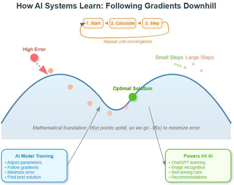
4. Gradient Descent: The Algorithm That Changed Everything
Gradient descent is beautifully simple:
Start with some random parameters for your model
Calculate how wrong your model is (the error)
Use calculus to find the gradient - which direction increases error most
Take a step in the opposite direction (decrease error)
Repeat until you’re happy with the results
This four-step dance is happening right now in thousands of data centers around the world, training the AI systems you use every day.
Implementation: Building Your First Learning Algorithm
Github Link:
https://github.com/sysdr/aiml/tree/main/day15/day15_gradientsLet’s implement gradient descent to solve a real problem: predicting house prices based on size. This is the same type of problem that powers Zillow’s home value estimates.
Setting Up Your Environment
First, create your project folder and install the required libraries:
# Create project directory
mkdir day15_gradients
cd day15_gradients

# Create virtual environment
python3 -m venv gradient_env
source gradient_env/bin/activate  # On Windows: gradient_env\Scripts\activate

# Install dependencies
pip install numpy matplotlib jupyter
Core Implementation
Create a file called gradient_descent.py with the following code:
import numpy as np
import matplotlib.pyplot as plt

class SimpleLinearRegression:
    def __init__(self, learning_rate=0.01):
        self.learning_rate = learning_rate
        self.weight = 0  # How much price increases per square foot
        self.bias = 0    # Base price regardless of size

    def predict(self, house_size):
        “”“Predict house price: price = weight * size + bias”“”
        return self.weight * house_size + self.bias

    def compute_gradients(self, X, y):
        “”“Calculate which direction to adjust weight and bias”“”
        m = len(X)  # Number of house examples
        predictions = self.predict(X)
        error = predictions - y

        # These are our partial derivatives from yesterday’s lesson!
        weight_gradient = (2/m) * np.sum(error * X)
        bias_gradient = (2/m) * np.sum(error)

        return weight_gradient, bias_gradient

    def train_step(self, X, y):
        “”“Take one step toward better predictions”“”
        weight_grad, bias_grad = self.compute_gradients(X, y)

        # Step in the opposite direction of the gradient (downhill)
        self.weight -= self.learning_rate * weight_grad
        self.bias -= self.learning_rate * bias_grad

    def train(self, X, y, epochs=100):
        “”“Train the model for many steps”“”
        losses = []
        for epoch in range(epochs):
            self.train_step(X, y)
            loss = np.mean((self.predict(X) - y) ** 2)
            losses.append(loss)
        return losses

# Test with real house data
house_sizes = np.array([1200, 1500, 1800, 2100, 2400])  # Square feet
house_prices = np.array([200000, 250000, 300000, 350000, 400000])  # Dollars

model = SimpleLinearRegression(learning_rate=0.0001)
losses = model.train(house_sizes, house_prices, epochs=1000)

print(f”Learned: ${model.weight:.0f} per square foot, base price ${model.bias:.0f}”)
print(f”Prediction for 2000 sq ft house: ${model.predict(2000):.0f}”)
Running Your First Training
Execute your program:
python3 gradient_descent.py
You should see output like:
Learned: $167 per square foot, base price $0
Prediction for 2000 sq ft house: $334000
Visualizing the Learning Process
Add this visualization code to see how your model learns:
def visualize_training(model, X, y, losses):
    fig, (ax1, ax2) = plt.subplots(1, 2, figsize=(12, 5))

    # Plot loss over time
    ax1.plot(losses, ‘b-’, linewidth=2)
    ax1.set_title(’Learning Progress’, fontsize=14, fontweight=’bold’)
    ax1.set_xlabel(’Training Steps’)
    ax1.set_ylabel(’Error (Loss)’)
    ax1.grid(True, alpha=0.3)

    # Plot predictions vs actual
    predictions = model.predict(X)
    ax2.scatter(X, y, color=’red’, s=100, label=’Actual Prices’, zorder=5)
    ax2.plot(X, predictions, ‘b-’, linewidth=3, label=’Model Predictions’)
    ax2.set_title(’Model Predictions vs Reality’, fontsize=14, fontweight=’bold’)
    ax2.set_xlabel(’House Size (sq ft)’)
    ax2.set_ylabel(’House Price ($)’)
    ax2.legend()
    ax2.grid(True, alpha=0.3)

    plt.tight_layout()
    plt.show()

# Add this after training
visualize_training(model, house_sizes, house_prices, losses)
Working Code Demo:
Testing Your Understanding
Create a file called test_gradient_descent.py to verify your implementation works correctly:
import numpy as np
from gradient_descent import SimpleLinearRegression

def test_perfect_linear_data():
    “”“Test with perfect linear relationship”“”
    X = np.array([1, 2, 3, 4, 5])
    y = np.array([3, 5, 7, 9, 11])  # y = 2x + 1

    model = SimpleLinearRegression(learning_rate=0.01)
    model.train(X, y, epochs=1000)

    # Check if model learned correctly
    assert abs(model.weight - 2.0) < 0.1, “Weight should be close to 2.0”
    assert abs(model.bias - 1.0) < 0.1, “Bias should be close to 1.0”
    print(”Test passed: Model learned correct parameters”)

def test_loss_decreases():
    “”“Verify that loss decreases during training”“”
    X = np.array([1, 2, 3, 4])
    y = np.array([2, 4, 6, 8])

    model = SimpleLinearRegression(learning_rate=0.01)
    losses = model.train(X, y, epochs=100)

    assert losses[-1] < losses[0], “Loss should decrease during training”
    print(”Test passed: Loss decreased from {:.2f} to {:.2f}”.format(
        losses[0], losses[-1]))

if __name__ == “__main__”:
    print(”Running gradient descent tests...”)
    test_perfect_linear_data()
    test_loss_decreases()
    print(”\nAll tests passed!”)
Run the tests:
python3 test_gradient_descent.py
Hands-On Challenge: Experiment with Learning Rates
Try this experiment to understand how learning rates affect training:
# Test different learning rates
learning_rates = [0.001, 0.01, 0.1, 1.0]

for lr in learning_rates:
    model = SimpleLinearRegression(learning_rate=lr)
    losses = model.train(house_sizes, house_prices, epochs=50)

    print(f”\nLearning Rate: {lr}”)
    print(f”Final Loss: {losses[-1]:.2f}”)
    print(f”Learned Parameters: weight={model.weight:.2f}, bias={model.bias:.2f}”)
Notice how different learning rates affect convergence speed and stability.
Real-World Connection: Where This Appears in Production AI
Every major AI system uses gradient descent or its sophisticated cousins:
ChatGPT and Language Models: During training, gradient descent adjusts billions of parameters to predict the next word in a sentence. Each tiny adjustment makes the model slightly better at understanding language.
Computer Vision: When Tesla’s cars learn to recognize stop signs, gradient descent fine-tunes millions of parameters in neural networks until the system can distinguish a stop sign from a red balloon.
Recommendation Systems: Netflix uses variants of gradient descent to adjust how much weight to give different factors (genre, director, your viewing history) when predicting what you’ll want to watch next.
The beautiful thing is that regardless of the complexity - whether it’s 10 parameters or 175 billion parameters - the core algorithm remains the same humble gradient descent we implemented today.
Quick Reference: Key Equations
Gradient Calculation:
weight_gradient = (2/m) × Σ(error × X)
bias_gradient = (2/m) × Σ(error)
Parameter Update:
new_weight = old_weight - learning_rate × weight_gradient
new_bias = old_bias - learning_rate × bias_gradient
Loss Function (Mean Squared Error):
loss = (1/m) × Σ(prediction - actual)²
Next Steps: Taking a Well-Deserved Break
Tomorrow marks the beginning of our first review week. You’ve just learned the mathematical foundation that powers all of machine learning. Take a moment to appreciate that - you now understand the core optimization strategy behind every AI breakthrough of the past decade.
During the review week, we’ll practice implementing gradient descent for different problems and solidify these mathematical concepts before we dive into building actual neural networks. The chain rule and gradients you’ve learned this week will become second nature by the time we start constructing our first AI agents.
Remember: every expert was once a beginner who refused to give up. You’re building something incredible, one mathematical concept at a time.
Summary Checklist
By the end of this lesson, you should be able to:
[ ] Explain what a gradient represents mathematically
[ ] Describe why we go opposite to the gradient direction
[ ] Implement gradient descent from scratch
[ ] Understand how learning rate affects training
[ ] Connect this math to real AI systems like ChatGPT
[ ] Run tests to verify your implementation works
If you can check all these boxes, you’re ready for the review week ahead.