

Today’s Agenda
Understand what PyTorch is and why it dominates modern AI research and production pipelines
Compare PyTorch’s dynamic computation graph to TensorFlow’s static approach
Install and configure PyTorch, then run your first tensor operations and neural network forward pass
Connect PyTorch’s design philosophy to the systems that power GPT-4, Llama 3, and Stable Diffusion
Why This Matters
You have spent the last several days building with TensorFlow and Keras. Now you are about to enter the framework that runs the majority of cutting-edge AI research today. PyTorch, developed at Meta AI Research, is the engine behind OpenAI’s GPT family, Meta’s Llama models, Hugging Face’s entire ecosystem, and most of the papers published at NeurIPS and ICML.
Understanding PyTorch is not optional for a serious AI engineer — it is the lingua franca of modern deep learning. More importantly, its design teaches you to think about neural networks in the way that actually helps you debug, optimize, and extend them.
Core Concepts
1. The Dynamic Computation Graph — Why It Changes Everything
Keras and early TensorFlow work by constructing a static computation graph: you define the full architecture, compile it, and only then run data through it. PyTorch works differently. It builds the computation graph on the fly, operation by operation, as your code executes. This is called a dynamic computation graph (or “define-by-run”).
Analogy: A static graph is a printed recipe you must follow exactly — no improvisation allowed. A dynamic graph is cooking live, adjusting ingredients as you go based on what you taste.
In practice, this means you can use normal Python control flow — if statements, loops, recursion — directly in your model logic. You can inspect intermediate values with a standard debugger. You can change the model structure between batches. This flexibility is exactly why researchers prefer PyTorch: experimenting with novel architectures is dramatically faster.
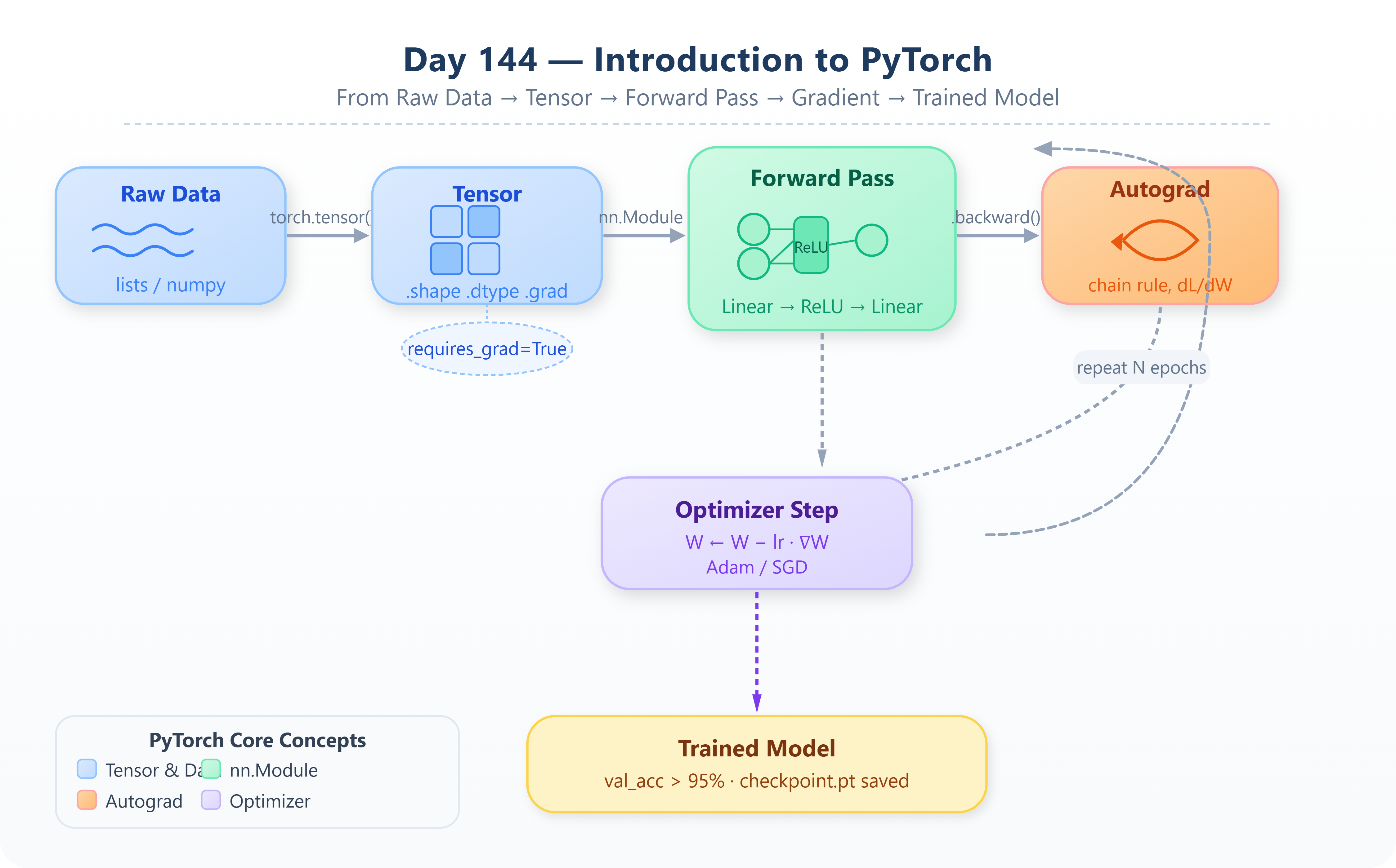
2. Tensors — The Core Data Structure
Everything in PyTorch is a tensor. A tensor is a generalization of arrays: a scalar is a 0-dimensional tensor, a vector is 1-D, a matrix is 2-D, and feature maps in a convolutional network are 3-D or 4-D. PyTorch tensors are nearly identical to NumPy arrays in API, but with two critical additions — they can live on a GPU, and they can track gradients for automatic differentiation.
import torch

x = torch.tensor([[1.0, 2.0], [3.0, 4.0]])
print(x.shape)   # torch.Size([2, 2])
print(x.dtype)   # torch.float32
When you move a tensor to GPU with x = x.to("cuda"), every operation on it executes on the GPU transparently. This single design decision is why PyTorch scales from a laptop to a 10,000-GPU cluster without changing your model code.
3. Autograd — Gradients for Free
The most important subsystem in PyTorch is autograd. When you mark a tensor with requires_grad=True, PyTorch silently records every operation applied to it in a directed acyclic graph. When you call .backward() on the loss, PyTorch traverses this graph in reverse, applying the chain rule at every node. You get gradients without writing a single derivative by hand.
w = torch.tensor(2.0, requires_grad=True)
loss = (w * 3 - 9) ** 2   # (6 - 9)^2 = 9
loss.backward()
print(w.grad)   # tensor(-18.)  —  d(loss)/dw
This is the same backpropagation you studied in earlier lessons, implemented automatically. Production systems at Tesla, Meta, and Google DeepMind all rely on this exact mechanism — just applied to networks with hundreds of billions of parameters.
4. nn.Module — The Building Block of Every PyTorch Model
PyTorch models are Python classes that inherit from torch.nn.Module. You define your layers in __init__ and implement the forward pass in forward(). This object-oriented design is not just stylistic — PyTorch uses the class structure to automatically register parameters, manage device placement, save and load checkpoints, and apply optimizations.
import torch.nn as nn

class SimpleNet(nn.Module):
    def __init__(self):
        super().__init__()
        self.linear = nn.Linear(4, 2)

    def forward(self, x):
        return self.linear(x)
Every production PyTorch model — from a two-layer classifier to a 70-billion-parameter language model — follows this exact same pattern.
Implementation — Build, Test & Demo
Github Link:
https://github.com/sysdr/aiml-p/tree/main/day144/day144_pytorch
The following steps walk you through building the lesson from scratch. Each step builds on the previous one. By the end, you will have a fully trained neural network, verified test results, and a saved model checkpoint.
Step 1 — Environment Setup
Before writing any model code, get PyTorch installed and confirm the environment is working:
pip install torch torchvision torchaudio --index-url https://download.pytorch.org/whl/cpu
pip install matplotlib numpy
python -c "import torch; print(torch.__version__)"
Expected output: 2.3.x or higher. If you have a GPU, run torch.cuda.is_available() to confirm it is detected. On CPU-only machines, everything in this lesson runs perfectly fine without any changes.
Step 2 — Tensor Operations
Create a file named lesson_code.py and begin by exploring the fundamental tensor operations. You will reference .shape, .dtype, and .device constantly when debugging production models, so become familiar with them now.
Implement and verify each of the following:
torch.zeros,torch.ones,torch.randn— tensor initializationtorch.matmul(a, b)— matrix multiplication (the core of every Linear layer)a.reshape(rows, cols)— reshape without copying data in memorya.to("cpu")/a.to("cuda")— moving tensors between devices
Step 3 — Autograd Walkthrough
Implement a manual gradient descent loop on a simple quadratic loss. Compute the loss, call .backward(), inspect .grad, update the parameter, then zero the gradient with w.grad.zero_(). Running 20 iterations should converge cleanly.
Pay particular attention to the underscore at the end of zero_() — in PyTorch, trailing underscores denote in-place operations.
Why zero the gradient? PyTorch accumulates gradients by default — each call to
.backward()adds to the existing.gradvalue rather than replacing it. If you forget to zero gradients before each iteration, your updates will be wrong. This is one of the most common bugs in beginner PyTorch code.
Step 4 — Build and Train a Two-Layer Network
Define a SimpleClassifier using nn.Module with two nn.Linear layers and a nn.ReLU activation. Generate synthetic data using torch.randn for features and torch.randint for labels. Then write the full training loop manually:
for epoch in range(100):
    optimizer.zero_grad()           # 1. Clear gradients from previous step
    outputs = model(X)              # 2. Forward pass
    loss = criterion(outputs, y)    # 3. Compute loss
    loss.backward()                 # 4. Backpropagation
    optimizer.step()                # 5. Update weights
This explicit loop — as opposed to Keras’s model.fit() — exposes every step of training. You control what happens before and after each gradient update. This control is precisely what you need when working with custom loss functions, gradient clipping, mixed-precision training, or multi-task learning.
Print the loss every 10 epochs and confirm it decreases monotonically.
Note: The five-line training loop above is what Andrej Karpathy — formerly OpenAI’s Director of AI — calls “the most important 20 lines in deep learning.” Understanding it at this level is what separates engineers who use AI from engineers who build it.
Step 5 — Verify, Test & Demo
Run the test suite to confirm everything is working as expected:
# Run from the day144_pytorch/ directory
pytest test_lesson.py -v
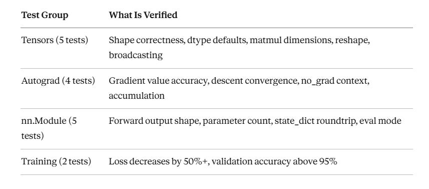
The test suite checks the following — all 16 tests should pass in under 30 seconds on CPU:
Component Architecture: PyTorch in an AI Agent System
In a production AI agent pipeline — say, a real-time document understanding service processing thousands of contracts per hour — PyTorch sits at the inference layer. Requests arrive via an API gateway, are preprocessed by a tokenizer or feature extractor (often NumPy or HuggingFace), and are batched before being passed to a PyTorch model loaded via torch.jit.script or torch.compile.
The data flow through the system looks like this:
API Request → Preprocessing → Tensor Batch → PyTorch Model (GPU) → Logits → Postprocessing → Response
PyTorch’s TorchScript mode compiles models into a portable intermediate representation that can be deployed without the Python runtime — enabling embedding models inside C++ services, mobile apps, or edge devices. Meta ships Llama inference to millions of devices this way.
The nn.Module you write today is structurally identical to the modules inside those systems. The training loop you write today is what Andrej Karpathy calls “the most important 20 lines in deep learning.” Understanding it at this level is what separates engineers who use AI from engineers who build it.
Real-World Connection
OpenAI’s GPT-4 training run, Stability AI’s Stable Diffusion fine-tuning pipelines, and Tesla’s Autopilot training infrastructure all run on PyTorch. The explicit training loop, autograd, and nn.Module pattern you practiced today are used verbatim — just at a scale involving thousands of A100 GPUs coordinated via torch.distributed.
The PyTorch team at Meta actively optimizes the framework for exactly these production workloads, making it the only framework where the gap between research prototype and production deployment is measured in days rather than months.