


What We’ll Build Today
Implement basic derivative calculations in Python for understanding gradient descent
Create functions that visualize how AI models “learn” through rate of change
Build a simple gradient calculator that shows how neural networks optimize themselves
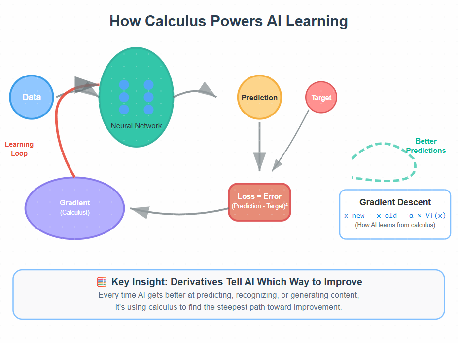
Why This Matters: The Mathematical Engine Behind AI Learning
Imagine you’re hiking down a mountain in thick fog, trying to find the lowest point. You can’t see far ahead, but you can feel the slope under your feet. Calculus is like that sense of slope—it tells AI systems which direction leads “downhill” toward better performance.
Every time you see an AI model improve its predictions, calculus is working behind the scenes. When ChatGPT generates better responses or when image recognition gets more accurate, it’s using derivatives to figure out how to adjust its internal parameters. Today, we’ll implement the fundamental calculus concepts that power this learning process.
Core Concepts: Calculus Foundations for AI
1. Understanding Derivatives as Rate of Change
In AI, derivatives tell us how much our model’s performance changes when we tweak its parameters. Think of it like adjusting the volume knob on a radio—the derivative tells us whether turning it clockwise makes the sound better or worse, and how quickly.
import numpy as np
import matplotlib.pyplot as plt

def simple_function(x):
    “”“A basic quadratic function: f(x) = x^2 + 2x + 1”“”
    return x**2 + 2*x + 1

def derivative_function(x):
    “”“The derivative: f’(x) = 2x + 2”“”
    return 2*x + 2
This derivative function tells us the slope at any point. In AI terms, it’s like having a compass that points toward improvement.
2. Implementing Numerical Derivatives
Real AI systems often deal with complex functions where we can’t easily write down the derivative formula. Instead, we approximate it numerically—the same way GPS calculates your speed by comparing your positions over time.
def numerical_derivative(func, x, h=1e-7):
    “”“
    Calculate derivative using the difference quotient method.
    This is how AI frameworks like TensorFlow compute gradients.
    “”“
    return (func(x + h) - func(x - h)) / (2 * h)

# Test our implementation
x_point = 3
analytical = derivative_function(x_point)  # Exact answer: 2(3) + 2 = 8
numerical = numerical_derivative(simple_function, x_point)

print(f”Analytical derivative at x={x_point}: {analytical}”)
print(f”Numerical derivative at x={x_point}: {numerical:.6f}”)
print(f”Error: {abs(analytical - numerical):.8f}”)
3. Gradient Descent: Following the Slope Downhill
This is where calculus becomes AI magic. Gradient descent uses derivatives to find the minimum of a function—exactly how neural networks learn to minimize their prediction errors.
def gradient_descent_1d(func, derivative_func, start_x, learning_rate=0.1, steps=50):
    “”“
    Implement basic gradient descent to find the minimum of a function.
    This is the core algorithm behind all neural network training.
    “”“
    x = start_x
    history = [x]

    for _ in range(steps):
        gradient = derivative_func(x)
        x = x - learning_rate * gradient  # Move opposite to gradient
        history.append(x)

    return x, history

# Find the minimum of our function
minimum_x, path = gradient_descent_1d(simple_function, derivative_function, start_x=5)
print(f”Found minimum at x = {minimum_x:.4f}”)
print(f”Function value at minimum: {simple_function(minimum_x):.4f}”)
4. Visualizing the Learning Process
Understanding how AI learns becomes clearer when we can see the process. This visualization shows how an AI system navigates toward optimal solutions.
def visualize_gradient_descent():
    “”“Create a visualization showing how gradient descent finds the minimum”“”
    x_range = np.linspace(-6, 4, 100)
    y_values = [simple_function(x) for x in x_range]

    plt.figure(figsize=(10, 6))
    plt.plot(x_range, y_values, ‘b-’, linewidth=2, label=’f(x) = x² + 2x + 1’)

    # Show the gradient descent path
    _, path = gradient_descent_1d(simple_function, derivative_function, start_x=4)
    path_y = [simple_function(x) for x in path[::5]]  # Every 5th step for clarity

    plt.plot(path[::5], path_y, ‘ro-’, markersize=6, label=’Gradient Descent Path’)
    plt.plot(path[0], simple_function(path[0]), ‘go’, markersize=10, label=’Start’)
    plt.plot(path[-1], simple_function(path[-1]), ‘ro’, markersize=10, label=’End’)

    plt.xlabel(’Parameter Value’)
    plt.ylabel(’Loss/Error’)
    plt.title(’How AI Models Learn: Following the Gradient Downhill’)
    plt.legend()
    plt.grid(True, alpha=0.3)
    plt.show()
Youtube Video:
Implementation: Building Your Calculus Toolkit
GitHub Link:
https://github.com/sysdr/aiml/tree/main/day12/day12_calculus_introLet’s create a complete toolkit that demonstrates how calculus powers AI learning:
class AICalculusToolkit:
    “”“A collection of calculus tools specifically for AI/ML understanding”“”

    def __init__(self):
        self.learning_history = []

    def loss_function(self, prediction, actual):
        “”“Simple squared error loss - what neural networks minimize”“”
        return (prediction - actual) ** 2

    def loss_derivative(self, prediction, actual):
        “”“Derivative of loss with respect to prediction”“”
        return 2 * (prediction - actual)

    def simulate_learning(self, initial_prediction, target, learning_rate=0.1, steps=20):
        “”“Simulate how a neural network learns to make better predictions”“”
        prediction = initial_prediction
        history = []

        for step in range(steps):
            loss = self.loss_function(prediction, target)
            gradient = self.loss_derivative(prediction, target)

            history.append({
                ‘step’: step,
                ‘prediction’: prediction,
                ‘loss’: loss,
                ‘gradient’: gradient
            })

            # Update prediction using gradient descent
            prediction = prediction - learning_rate * gradient

        return history

    def explain_learning_step(self, step_data):
        “”“Explain what happened in a learning step”“”
        return f”Step {step_data[’step’]}: Predicted {step_data[’prediction’]:.3f}, “ \
               f”Loss: {step_data[’loss’]:.3f}, Gradient: {step_data[’gradient’]:.3f}”

# Demonstrate AI learning
toolkit = AICalculusToolkit()
learning_process = toolkit.simulate_learning(initial_prediction=8.0, target=3.0)

print(”AI Learning Process:”)
for i in [0, 5, 10, 15, 19]:  # Show key steps
    print(toolkit.explain_learning_step(learning_process[i]))
Real-World Connection: Calculus in Production AI
Every major AI system uses these calculus concepts:
Neural Networks: Use backpropagation (chain rule of calculus) to learn from mistakes. When GPT-4 generates text, it’s using derivatives to adjust billions of parameters.
Computer Vision: Image recognition models use derivatives to detect edges and features. Self-driving cars use calculus to track moving objects.
Recommendation Systems: Streaming services use gradient descent to learn your preferences and suggest content you’ll enjoy.
The simple gradient descent we implemented today is the same fundamental algorithm used in training systems like GPT, DALL-E, and autonomous vehicles—just scaled up to work with millions of parameters instead of one.
Next Steps: Building on Our Foundation
Tomorrow in Day 13, we’ll explore derivatives and their applications more deeply. We’ll learn about partial derivatives (for functions with multiple inputs) and see how the chain rule enables neural networks to learn complex patterns. You’ll implement backpropagation from scratch and understand exactly how deep learning systems train themselves.
The calculus foundation you’ve built today will make those advanced concepts feel natural and intuitive. You’re now equipped with the mathematical intuition that separates AI practitioners from those who just use AI tools—you understand how the learning actually happens under the hood.
Regarding the topic, I always find it absolutely fascinating how calculus provides such an elegant engin for AI's learning and optimisation.